How effective are different parts of California at addressing homelessness?
At Real Good AI, we want to use data science to learn more about the world in a way that could help people and make it better with that science. One of our nonprofit partners, California Elder Justice Coalition, is already working on advocating for justice for the unhoused elderly in California.
California has a disproportionate share of the United States' unhoused population. In 2024, the state accounted for 24% of the nation's total homeless, despite having only 12% of the population [1]. It’s like California is pulling a double shift for the rest of the country. This crisis has worsened in recent years, with the number of people experiencing homelessness increasing by 6% between 2020 and 2022 [2]. In the scientific literature, this growth is largely attributed to systemic factors, particularly a severe housing affordability crisis where housing costs have outpaced supply and incomes [1], [3]. While California has invested significant funds into programs aimed at reducing homelessness, a statewide audit noted a lack of information to assess the effectiveness of these programs, highlighting a need for evidence-based evaluation [1]. It is hard to know what to advocate for without knowing which programs are the most effective or even if they were making any change at all!
We thought we could use some basic models (with a fun twist) to help them answer most specifically: Where is the unhoused population larger or smaller than we expected? Then we pass that information to them to try and discover the bigger question: WHY?
Let’s break our analysis down:
STEP 1: Assemble the data
STEP 2: Predict what we know (build the model)
STEP 3: Predict what we don’t know (use the model)
Fortunately, evidence is available in the form of public data! So let's take a closer look at the data available and try to measure the effectiveness of different parts of California at addressing homelessness. We hope you enjoy this summary of our work and learn just a little bit about the process of building a stats model!
STEP 1: Assemble the Data
We combined data from a few open-source publicly available sources into one big dataset for our analysis.
The most important piece of data is the Homelessness count by age dataset available on the California Open Data portal. This dataset is compiled from the Homelessness Data Integration System (HDIS), which aggregates information from service providers across all 44 California Continuums of Care (CoCs) [2]. The CoCs are the regional bodies responsible for coordinating local homelessness responses and will be our unit of analysis. Think counties, but this is a little bit more general of a term. The data covers the period from 2017 to 2023. The data primarily captures individuals who interact with the formal service system so it may undercount the total unhoused population, particularly unsheltered individuals who do not access services.
We want to figure out how homelessness counts are related to other variables. In the language of statistics, the homelessness counts represent our dependent variable because it depends on a number of other variables: the independent variables. We also call them features.
Several factors (or independent variables) can influence the number of unhoused people in a given region. First and foremost is the total population of the region, our first independent variable. Population figures were sourced from the U.S. Census Bureau, including American Community Survey (ACS) estimates and Decennial Census data. Another important factor is the housing cost for the region. We used the Zillow Home Value Index (ZHVI) for all homes (including single-family residences, condos, and co-ops), using the smoothed, seasonally adjusted time series [6]. We also included some geographical information about CoCs from the U.S. Department of Housing and Urban Development [7].
Most unique to our analysis, we incorporated the spatial location of a region in two ways. Anyone who has been to California will tell you the coast is SO DIFFERENT than further inland. Similarly, the vibe and weather in Northern and southern CA are very unique. So we can readily extract the latitude and longitude of the centroid of each region’s shape.
Next, if there is something positive or negative going on right next to a region, we expect there to be some spillover into regions right next to it. So we can define the neighbors of each region. This adjacency data allows us to define a new spatial lag variable containing the population-weighted average homelessness count of neighboring regions.
Lastly, since statistical models are computing numbers, we need to somehow convert our data into something we can use. For example, the age group category for unhoused people is a grouping rather than a number we can input. This is actually a super common issue that arises in data science so we wanted to explain it a little more here. For that we use a conversion method called one-hot encoding. Basically, we rearrange the variables so that instead of one variable that contains group 1, 2, 3, 4, 5 etc. we have a series of variables that each have 0/1 ONLY. Just think about it, we totally made up the ordering of the groups in the 1, 2, 3, 4, 5 labeling so we need a way to separate them each out. Then, each of these new variables asks: Do they belong to group 1? Group 2? Etc and answer 0 for no and 1 for yes accordingly. Then we can interpret the results of each of these variables as the effect of being in that group.
STEP 2: Predict What We Know
Our goal is to build a statistical model trained on the data we have and can make predictions based on new data. This is called regression. In this particular case, the model must predict homelessness counts of a region given the region's population, cost of living, spatial lag, latitude, and longitude for a given year and age group.
In theory, one could use a model like this to extrapolate data, for instance to a future year for which we have no data. But extrapolating isn't that useful here because we wouldn't be able to verify the model's prediction against actual data. A trick often used in machine learning when developing models is to split the data you have into a large training set and a smaller test set. This lets you compare your predictions of the test data with the actual data that was withheld from training to assess the quality of the fit.
There are several choices of models for doing regression. Here we choose a Random Forest model for its strength in capturing complex, non-linear relationships and interactions between variables. Think of a Random Forest as the averaging of a bunch of simple models. We at least know why it makes decisions and how many of the smaller models made those decisions so it isn’t the total black box of other machine learning options.
OK, ignore this if computer code scares you! Here is what the splitting, fitting, and prediction looks like in Python:
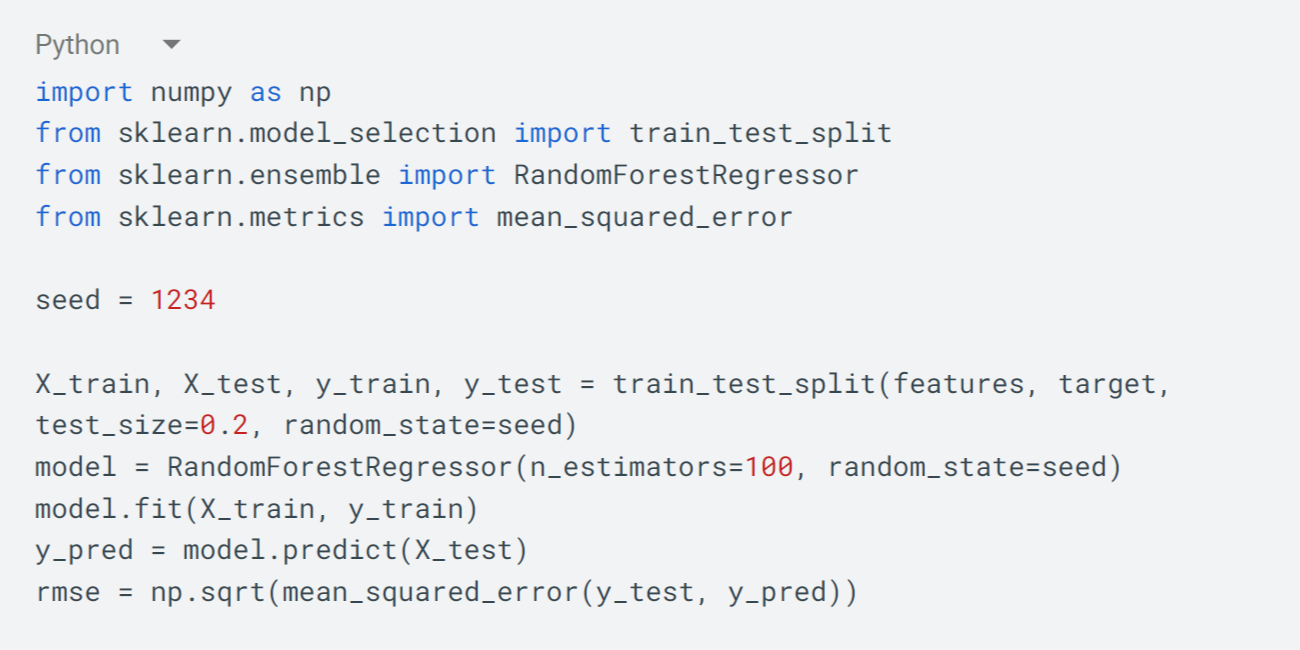
Beyond ensuring we have a good fit by computing the Root Mean Squared Error (RMSE) between the predictions and actual test data, we can also interrogate the model about the relative importance of different features.
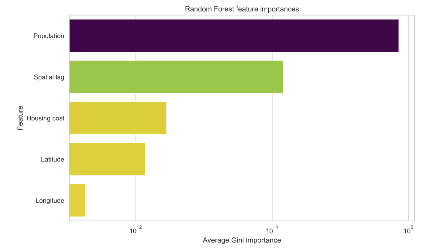
We see that population is by far the main predicting factor of homelessness count in a given CoC (note the log scale).
STEP 3: Predict What We Don’t Know
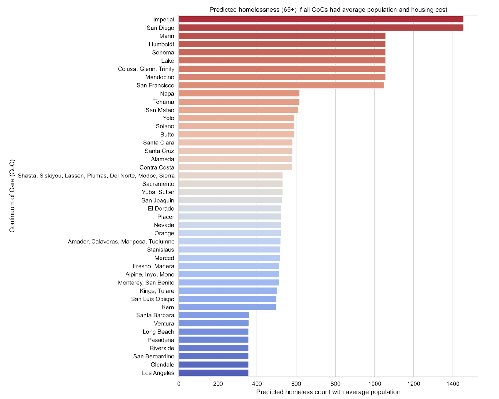
We now have a way to predict what we already know, which doesn't sound that impressive, but now we get to do what we set out to do! As the title suggests, we're interested in answering how effective are the different CoCs at addressing homelessness. In particular, we would like to control for external factors that are outside of the CoCs control. For instance, as we've seen, population is a major factor, so to level the playing field, we build a new dataset where we pretend that all the CoCs have the same population, equal to the statewide average population. Then we follow the same steps as before to fit a model on that artificial dataset. This time, we're no longer predicting actual homelessness counts for each CoC but the numbers we're predicting are comparable between CoCs. By substituting the three most important features which are population, spatial lag, and housing cost, we can predict how each CoC fares at reducing homelessness when ignoring those external factors.
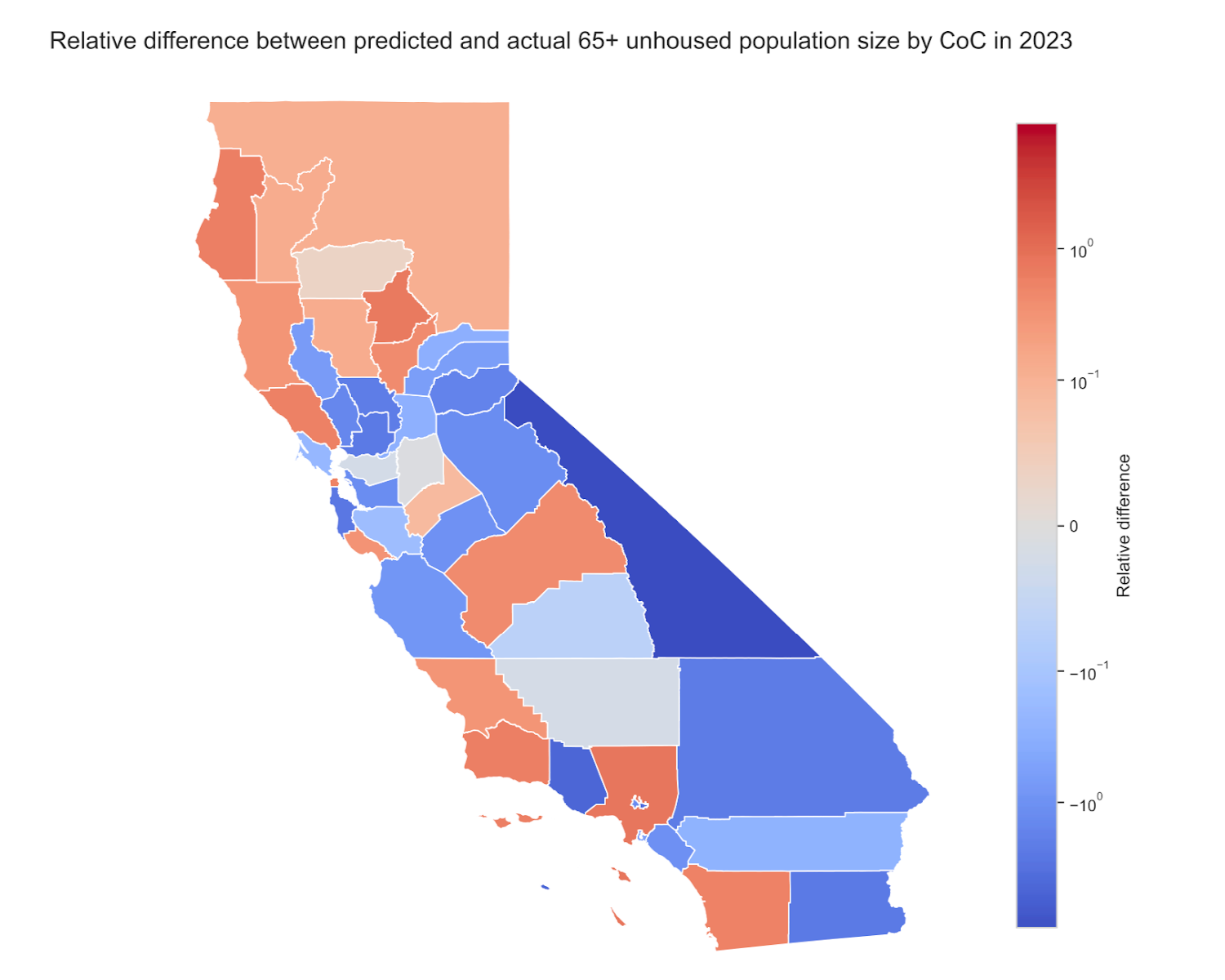
You can read this plot like you'd guess: red areas have more unhoused individuals than expected, while blue areas have fewer than expected. Our analysis suggests that LA county CoCs, despite being a hot spot for homelessness due to their high population and housing costs, are managing the crisis more effectively than other CoCs in less populated areas. Conversely, some areas seem to be underperforming relative to their potential. These are the areas where policymakers should consider new approaches.
A Word of Caution
We are in fact humans so there was only so much time when we did this analysis. If we lived outside of space and time, there are several ways in which this analysis could be improved. Firstly, there are many other external factors that could be considered to be included in our model, like unemployment, urbanization, weather, and other socioeconomic factors. Our current predictions are obviously limited to the data we use to fit the models. Finding and processing public data takes time and effort but could potentially lead to better insights.
Secondly, flagging anomalies doesn't explain why the anomalies exist. To really get to the causes, we would need to look at things like funding for CoC operations and specific housing policies. We leave this to our partners and to future scientific study to really understand the “why” behind these anomalous answers. Maybe you know? We’d love to hear from you if you do!
Conclusion
We can't fix what we can't measure. Public data is a blessing. It can be a lot of work to collect and curate data from many different sources, but it's a rewarding journey when, coupled with powerful statistical AI tools (you might say real good AI tools), we can gather insights and hopefully help out our communities. Informed policy is essential to a well-functioning society. We hope you enjoyed our data journey and will come along for the next ride from the Real Good AI team!
[1]: https://www.ppic.org/blog/homelessness-hits-record-high-in-california-jumps-dramatically-in-rest-of-us/
[2]: https://bcsh.ca.gov/calich/hdis.html?utm_cta=website-nav-resources-office-hours
[3]: https://www.huduser.gov/portal/publications/Market-Predictors-of-Homelessness.html
[4]: https://data.ca.gov/dataset/homelessness-demographics
[5]: https://www.census.gov/data.html
[6]: https://www.zillow.com/research/data/
[7]: https://www.hudexchange.info/programs/coc/gis-tools/
[8]: https://en.wikipedia.org/wiki/One-hot