Gaussian Process Diffusion
It’s a well known fact that AI-generated images are based on data taken without the creator’s consent. Once the models are trained, the model doesn’t make direct reference to the data. This fact provides the argument that the model itself is being “transformative”, but that doesn’t stop AI models from being labeled "plagiarism machines” by the online public. The truth of the matter is somewhere between, where data is guiding generation through shaping the model, but it is unclear how. But what if there was another way? A way to respect the rights of and provide credit and possible payment to any artists who would participate in training data in the future? A way to attribute the contribution of those creators in specific generated images? This was the challenge I aimed to tackle during my first days with Real Good AI. My thinking was this: not everything about the neural network approach that led to the “black box” problem that keeps us from knowing where its generated images are coming from needs to be discarded. The general process of how the images get generated was not the problem, but instead the model that’s generating is what needed to be replaced. The answer to this replacement problem was straightforward given the proclivities of the Real Good AI research team: I should try combining the “diffusion” process of neural network image generators with the Gaussian Process (a.k.a. the “GP”).
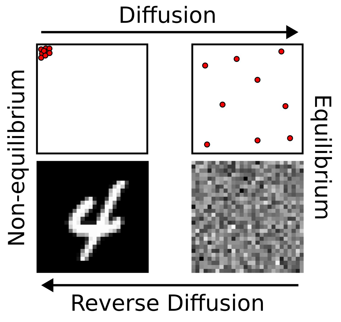
Imagine a group of balls densely packed in one corner of a box. Now, give them all a random direction of movement and let them bounce around the box like a bunch of DVD logo screensavers. Eventually, the balls will become (approximately) evenly dispersed inside the box. This process is called “diffusion” in science, and represents the process of the balls from going from a state of disequilibrium (“bunched up”) to equilibrium (“evenly spaced”). In an AI image diffusion model, diffusion comes in the form of a transition from the “disequilibrium” of an image to the “equilibrium” of random noise. But wait, isn’t the model supposed to be making images, not noise? This is because what a diffusion model actually learns is reverse diffusion, the process of predicting the denoised image from “diffused” noise. In our metaphor, we are putting the balls back in the corner. In practice, this means our model learns how to make a clear image from what once was noise.
There’s a couple different ways to implement a diffusion model, the simplest of which is to predict what the fully denoised image will look like given the current image and taking a small step towards it until the image looks clear. This is the method I used in implementing my diffusion model, as it seemed to work better than the alternatives . This means that the training data set we’ll be using in our models consists of the original image with random amounts of noise added, representing different paths and timescales of diffusion from the initial image. The model then learns to predict the original clear image from each of these “timesteps” of the diffusion process. The number of steps the model will take to go from full noise to generated image is specified as part of the script, where more steps gives a higher quality final image but also requires a longer runtime.
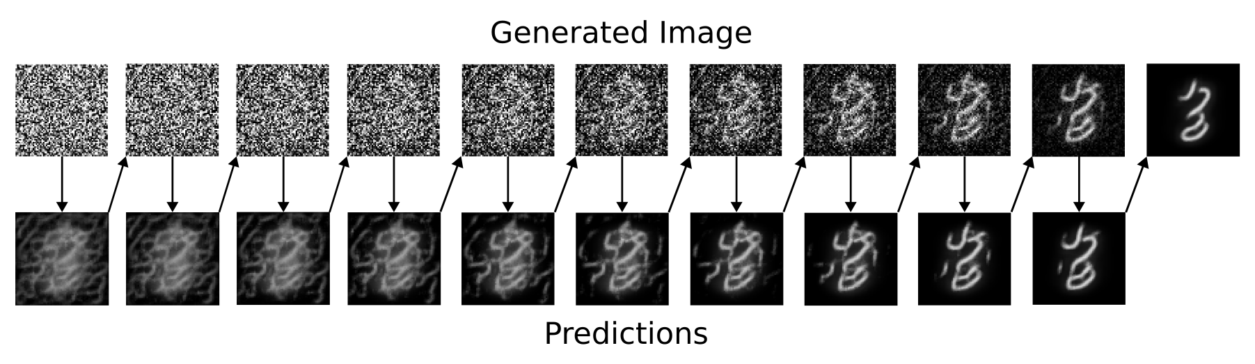
Starting from white noise, which is like snow on a bad TV channel (top left), we guess what the image could look like (bottom left). We move a little bit towards that image and try again. We repeat this over and over as many times as we would like until we have a clean looking image.
So then what did you do differently?
You may have noticed by this point that I haven’t mentioned how the GP changes anything about the diffusion model. After all, aren’t we supposed to be going away from neural networks? This is because the diffusion model framework we described does not inherently imply that a neural network has to be what is trained; anything can be used to learn the prediction of the denoised image from noise. So why is the GP any better than a neural network for that? The secret is in the math under the hood between the two models. In a neural network, the training data is used to optimize a set of weights so that the error of the predictions of the network is minimized. But once training is over, that training data mathematically disappears, and all that’s left is the “vibe” the neural network got from it in the form of its weights. GPs are different because they use the training data directly every time they make a prediction. What this means is that if you predict using a GP, you can see exactly which training data was used to formulate that prediction. In terms of AI generated images, if you use a GP instead of a neural network to generate images, you can literally point to which images in the training data were used to generate it and give proper attribution to those images in your final product. While formalizing this attribution part is still being worked on as a direction of research at Real Good AI, it definitely motivates us to see how well the GP works for diffusion.
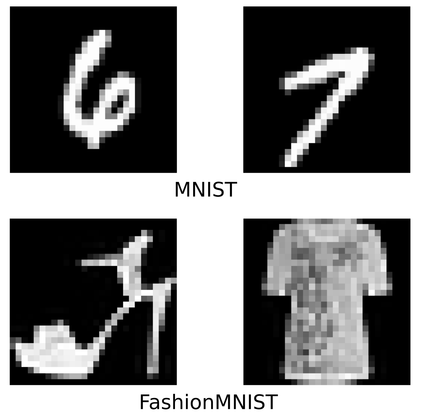
My first attempt at making a GP diffusion model was to have it generate based on the entire image, where the number of pixels of noise it was going to denoise was the same number of pixels in the images of the training data. I tried training the model to generate images from two datasets: 1. The famous MNIST image dataset of handwritten numbers 2. The less famous fashionMNIST dataset of clothing items. I chose these datasets because they’re well-studied and well standardized (every image is a 28x28 grayscale image with a known label). However, the result from this initial model ended up being relatively uninteresting, as it ended up generating images that were almost exact replicas of the training data. In other words, the diffusion model would end up choosing a single image from the training data early on that it thought the final image would become, and then never change that guess for the rest of the generation. Also, the fact that we could only make images the same size as the training images seemed like a pretty annoying limitation. So clearly, we needed to take a different approach to how we were structuring the input.
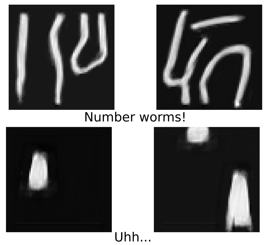
The next version of the model came from an operation used frequently by neural networks to solve this problem: convolution, or in other words, using a “sliding window” approach to denoising the image. With this strategy, instead of the entire image being denoised all at once, each pixel would get denoised according to the pixels that were immediately surrounding it, making the generation process much more locally focused than before. Since the window was able to “slide” along each axis as far as it wanted, this meant that images could now be made in any size. Pixels that were near the edge of the image had “padding” of zero values tacked on to them to make sure the window could reach every pixel of the image. The main result of this “convolutional” approach was to start generating what I referred to as “number worms” in the MNIST dataset. These “worms” were exciting to see because they were clearly unlike anything in the training dataset but had features derived from it, such as the turns of a 0 or the bottom of a 4.
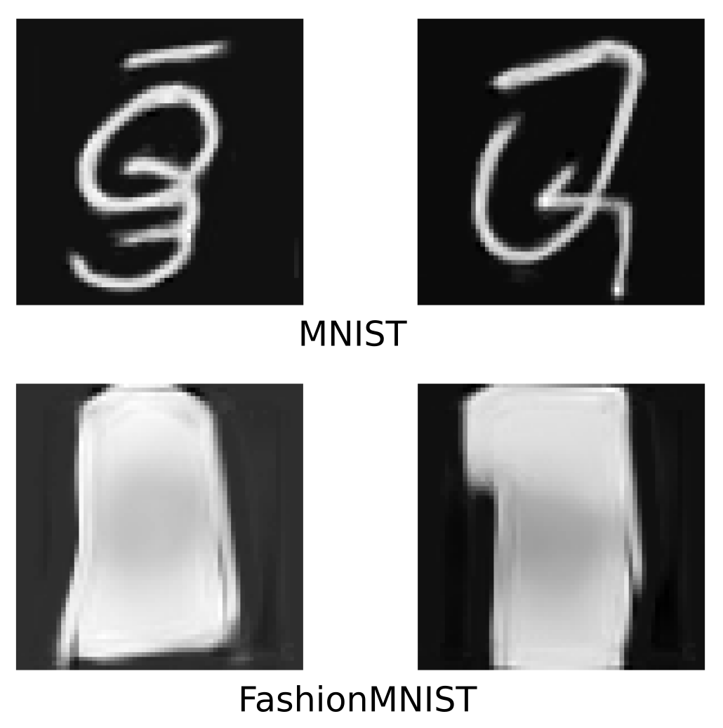
While the worms were a step in the right direction, the battle was far from over. These worms came to be because they were a compromise between a bunch of overlapping windows all trying to have their say into what the image should look like. This becomes even more clear when we jump to the fashionMNIST dataset where every generated image of clothing comes out as a very fashionable streaked pattern. So how can we get the windows to fight less about their vision for the image? The solution that I arrived at was to add a positional embedding to the inputs of the model, or in other words, telling the model the part of the image it was cleaning up This change seemed to solve the problem, as it thinned out the number of choices each window could make to denoise the image. By thinning out the landscape of choices each individual window could make, the windows were able to come to more clear consensus on what shape the pixels should take and begin to generate some really unique shapes. However, since the generation process was so local, different regions of the image could be making their own version of the image that eventually gets stitched together instead of producing one coherent image.
The “small tweak” that took a month to figure out
As one often does in research, I made a small tweak to the methodology. This significantly improved performance for pixel value prediction, and made the model much more robust to different amounts of noise. However, the generation quality did not improve, with MNIST resulting in a chaotic spaghetti of lines and fashionMNIST creating a giant brick of washed-out grey. This change to the model made enough logical sense that I didn’t want to just roll back to the previous model; finding out how to fix this problem would prove to be an obstacle that would last the next month’s work of research.
After thinking about the mathematics of the model, I had deduced that the source of the problem was the very thing I sought to attain: more robust outputs meant a lack of diversity in predictions from almost pure noise. So then how do we fix this disconnect between what’s good for prediction and what’s good for generation? Surprisingly, the solution is very similar to what got us away from number worms: encode the position of prediction more strongly into the model. After all, the problems are quite similar in that they originate from the model having too many equally good directions for denoising the image. To accomplish this, I first separated the length-scale parameters of the positional embedding to be separate from the length-scale of the image input so a change in position could be learned to be more or less important than a change in input pixels if necessary. I also introduced a new secondary GP to predict the average pixel value based on image position so the denoiser had a more reasonable baseline to predict from.
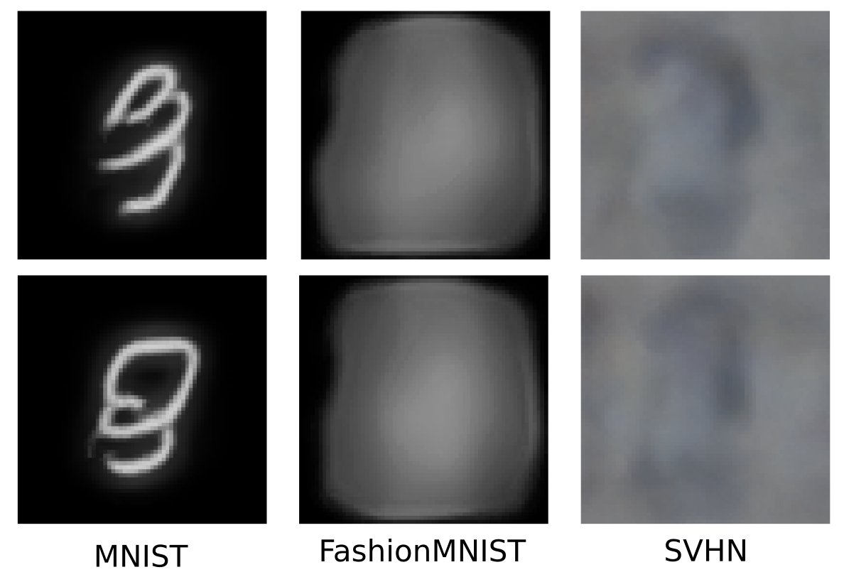
While this is very close to the final model posted on our github (https://github.com/Real-Good-AI/GPDiffusion), there was one more problem I identified that I wanted to address before stopping: the parameters of the GP shouldn’t be the same at every timestep of the denoising. It would make sense that noisy inputs would require longer lengthscale parameters and larger measurement error parameters than inputs that are close to being fully denoised. Therefore, these parameters are not fit as a single value, but instead are predicted through a linear regression based on the variance of the input. A few other details were tweaked relative to the previous model, such as more properly implementing the denoising schedule and reclustering training set examples to ensure nonredundancy. Given all these tweaks, we arrive at the final version of the model, whose generations on the two datasets we discussed previously are presented below. We also present generations in color using a dataset of house numbers from Google Street View (Street View House Numbers, SVHN).
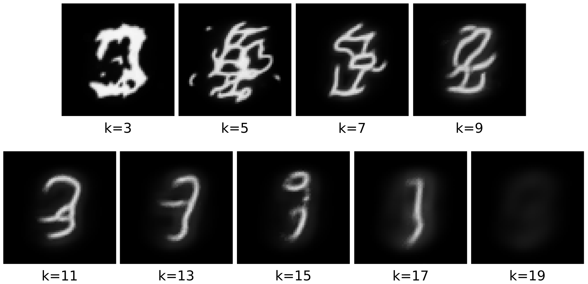
To show how the size of the convolutional window impacts image generation, here’s a set of emacs images generated with increasing sliding window size (k is the number of pixels on one side of the window).
Where is the project now?
To be honest, this project is still buried under a lot of important questions. First, how do we get one part of the image to “talk” to another part of the image mid-generation if the sliding window approach is so local? In neural networks, this is solved by layering, but GPs are unable to layer in their purest form due to their inability to make arbitrary “hidden” spaces like neural networks do. There have been attempts to address this shortcoming of GPs (“deep” GPs), but these methods tend to obfuscate the attribution advantage we’re trying to leverage. Also, more modern neural network solutions for diffusion usually also incorporate some version of the attention mechanism to allow the model to “see” pixels across the entire image when making decisions. Both of these ideas have been incorporated into our GP transformer model (article on this coming in the future!), but the way that deep GPs are implemented in that model destroys the data attribution component that was so valuable about this architecture. Another question is how do we scale up the size of images we want to generate and number of training examples without overloading memory? And how best can we extract attribution from the GP given the diffusion process? These are questions currently being researched by Real Good AI, where we aim to fit GPs to existing neural networks so we can reverse engineer data attribution from already popularly used models if we know their training dataset. Once we make significant progress answering these questions, we’re hoping to return to this diffusion model and take it to a place that can rival existing neural network based models, but with the significant advantage of giving credit to the art and artists who fuel this genre of models.
(almost) all figures have images generated by our model